Multi-neuron Analysis
Regarding a method to interpret multiple neurons simultaneously.
[📚 Neuron Series 3]
Introduction
Deep neural network has lots of parameters in its module. When we group parameters by the minimal meaningful components, we can consider a concept neuron which is known to have meaningful concepts or patterns
Multi-neuron in Linear Layer
In this post, we only handle multi-neuron in a linear layer as most complex modules are the mixture of linear layers. If you require preliminaries on neurons in a linear layer, please check this [post]. The summary of multi-neuron in a linear layer is as follows
- a neuron in a linear layer is each row
- the number of neurons in a linear layer is the size of row
- the number of synapses (connections) is the size of column
The multi-neuron that we consider is $m$ neurons with $n$ synapses which interpret $n$-dimensional input.
Interpretation of Multi-neuron
With a definition that column size is the processed information dimension for each neuron, we only consider size 1 and 2 dimensional size input as larger than 3 dimensional size input could not be visualized.
The Figures below show two neurons which process 1D input and 2D input. We represent each entry of input as F and the neuron’s output with A. In addition, we use red color for positive output and green color for negative output
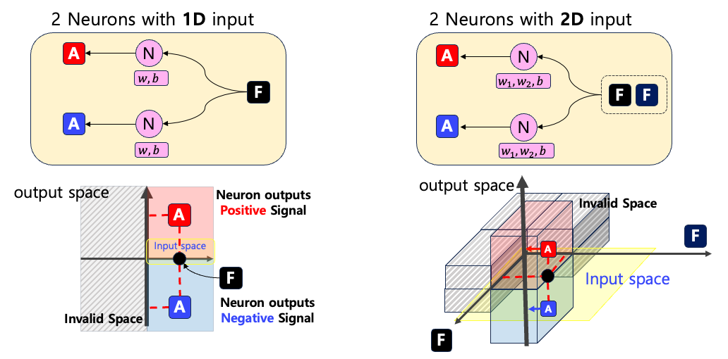
F for 1D input or FF for 2D input). The yellow regions are input regions and we consider only positive regions Note that these visualizations require +1 dimensional space of input space as a neuron output scalar. This is why we can interpret maximally multiple neurons with 2D input size as the visualization requires 3D space. We said that a neuron can output either positive or negative scalars. We analyze the change of signs as it highly affects the behavior of neurons. Optionally, we can analyze the output of neurons with 95% quantiles. That is, we analyze whether a neuron gives a high scalar for an input or not.
Visualization of multi-neuron
In this section, we provide visualization results of neurons for all positive input values. We use random weight $W \in \mathbb{R}^{8\times1}$ and bias $b \in \mathbb{R}^{8}$. In this case, the number of neurons is 8 and the input dimension is 1. In addition, we specifically highlight two cases, Input 1 and Input 2.
-
input 1is small signal 0.3 -
input 2is large signal : 0.7
The visualization shows individual neurons as a line
\(y = w_n x +b_n\)
where $x$ is the input and $y$ is the output of the neuron which has weight $w_n$ and bias $b_n$. These lines are guidelines to show how neurons give outputs. For input 1 and input 2, you have to check only $x=0.3$ and $x=0.7$ respectively.
Input Boundary
In the previous section, we described the change of sign for outputs. This observation remains the following question on the input regions. Can we dissect input regions and discover meaningful regions? This question is naive but related to more interesting problems. For example, CLIP
We partition the input space with the sign of the output for neurons. With the Figure below, you might notice that the partitioned regions are determined by the points of intersection. In addition, at each point, the behavior of a neuron could be increasing or decreasing which is determined by the slope of a line (sign of weight). Therefore, for the clear description, we should visualize two things
- The points of intersection (📐)
- The sign of slope (🔴, 🟢)
To this end, we have the following visualization of neurons and input boundaries for 1D input.
You can visualize only the input region removing the guidelines of neurons.
2D
Now we visualize 2D input space in which a neuron has a single output, and in total requires 3D visualization for neuron behavior. The visualization technique is the same with the case of 1D visualization. The only difference is that now a boundary is a line instead of a point and a guideline for a neuron is a plane instead of a line. The Figure below shows visualization of random neurons with projection on the xy-plane (a region where the sign of a neuron changes).
Similarly, we can visualize the input boundaries without the guidelines. We visualize the green region as the region where the neuron’s output is positive and the red region as the region where the neuron’s output is negative. With this visualization technique, we can interpret the signs of two Regions (Skyblue and Magenta).
Such a visualization provides a much deeper understanding of input regions. Imagine that we have an input in Region1 and move it to Region2. With such a change we expect the positive output of Neuron 1 as the color goes from Red to Green.