Neurons in Deep Learning
How can we interpret neurons in deep learning?
[📚 Neuron Series 2]
Introduction
In the previous section, we introduced neurons in deep learning by comparing neurons in neuroscience. The previous section only introduced neurons in a linear weight and bias. With the same interpretation, we introduce several neurons in deep learning modules including multi layer perceptron (MLP), convolutional neural network (CNN), recurrent neural network, and generative pretrained models (GPT). In addition, we also provide a neuron perspective on key-value memory in GPT. We believe this interpretation of neurons can further help to understand the general computation of deep neural networks.
Linear Neurons in MLP
Let see the most basic module, weights in a linear layer. The weights are a matrix whose rows are the outputs for neurons and the columns for the synapses of these neurons. You can think that each row (neuron) computes independently the input signal $x$.
With the assumption that $W \in \mathbb{R}^{\textcolor{red}{m} \times \textcolor{blue}{n}}$
- 🌱 number of neurons : $\textcolor{red}{m}$
- 🌱 number of synapses per a neuron : $\textcolor{blue}{n}$
- 🌱 number of synapses in total : $\textcolor{red}{m} \times \textcolor{blue}{n}$
MLP is a series of linear neurons with activations in between them. The activations are thresholds to pass the information with valid signals. For example, ReLU cuts negative signals and Tanh provides gating mechanisms of signals. Therefore, in the interpretation of neurons, we can think of activations as modifiers of neurons’s outputs.
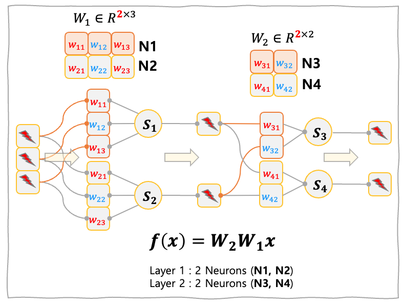
The Figure below shows two layer MLP. Each layer has two neurons and the neurons in the first layer have three synapses for each neuron, while the neurons in the second layer have two synapses for each neuron.
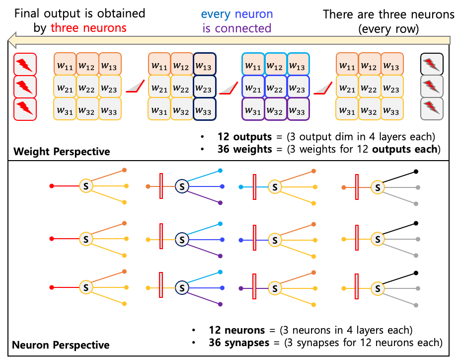
The Figure below shows the four layer MLP. In each layer, three neurons exist and each neuron has three synapses. Note that all the pre-neurons and post-neurons are connected with synapses. We think that is why MLP is called a densely connected neural network.
Convolutional Neuron
Convolutional layer is also considered as a linear layer as we can reformulate the convolution operation as a linear operation. However, we use another tool to interpret the convolutional neuron. The most frequent way of creating a convolutional layer is using the notation: (out_channels, in_channels, kernel, kernel, ..). With this notation, the out_channels parts are the same with the rows in the linear neuron and (in_channels, kernel, kernel) are the synapses for a neuron. With this interpretation, the only difference with the linear layer is (kernel, kernel) part where the convolution operation is applied in the 2D plane. If you assume that kernel size is 1, then you can think of a linear neuron!
- 🌱 number of neurons :
out_channels - 🌱 number of synapses per a neuron :
in_channels$\times$kernel$\times$kernel - 🌱 number of synapses in total :
out_channels$\times$in_channels$ \times$kernel$\times$kernel
Recurrent Neuron
Beside MLP and CNN, the other basic module is a recurrent neural network (RNN) which successively computes an input with linear operations in it with hidden states. Computationally, the recurrent neuron is the same with the linear neuron except input and output types. Note that the recurrent neuron should provide outputs which are re-injected to the input of that neuron. The advanced RNN modules such as LSTM
Neurons in GPT Block
Now we discuss neurons in more advanced architectures such as GPT. GPT consists of a token embedding module, transformer decoder blocks and task specific heads such as LMHead. We verify neurons in a GPT block and leave the interpretation of other modules as they are just linear-like neurons. GPT block has two main parts MLP and self-attention (or cross-attention), and layer-norm.
MLP
MLP block is a two layer MLP whose first layer is sometimes called key and second layer sometimes is called value. We use $d_{model}$ which is the dimension of GPT representations to describe the number of neurons and synapses. The key part is a linear layer with weight \(W_{key} \in \mathbb{R}^{\textcolor{red}{4\cdot d_{model}} \times \textcolor{blue}{d_{model}}}\) whose number of neurons is four times larger than the number of synapses. On the other hand the value part is a linear layer with weight \(W_{value} \in \mathbb{R}^{\textcolor{red}{ d_{model}} \times \textcolor{blue}{4\cdot d_{model}}}\) whose number of neurons is four times smaller than the number of synapses. Therefore, this architecture is a bottleneck architecture and many researchers interpret it as a neural memory.
Consider $d_{model} = 12,288$ which is the hidden dimension size of GPT3 (175B).
- 🌱 number of neurons : 49,152 (key neuron) + 12,288 (value neuron)
- 🌱 number of synapses per a neuron : 12,288 (key neuron), 49,152 (value neuron)
- 🌱 number of synapses in total : 1,207,959,552
(= 49,152 $\times$ 12,288 (key neuron) + 12,288 $\times$ 49,152 (value neuron))
ATTN
In ATTN, there are four linear layers: query, key, value, output and each layer has weight \(W \in \mathbb{R}^{\textcolor{green}{d_{model}} \times \textcolor{green}{d_{model}}}\). Therefore, we can easily interpret neurons in ATTN
Consider $d_{model} = 12,288$ which is the hidden dimension size of GPT3 (175B).
- 🌱 number of neurons :61,440 = 12,288 $\times$ 4 (Q, K, V, O)
- 🌱 number of synapses per a neuron : : 12,288 (Q, K, V, O)
- 🌱 number of synapses in total : 603,979,776 = (12,288 $\times$ 4) $\times$ 12,288
Neurons in GPT3 (175B)
Finally, we count the number of neurons and synapses in GPT3 (175B) blocks with the above interpretation
- 🍀 (
GPT3) number of synapses : 173B
(173,946,175,488 = 96 $\times$ (1,207,959,552 + 603,979,776))2B difference (175B and 173B) is due to bias, embedding, layer-norm and LM heads modules. - ☘️ (
GPT3) number of neurons : 11M
(11,796,480 = 96 $\times$(61,440+61,440)) - ☘️ (
GPT3) number of synapses per a neuron : 14,745
As humans have 7,000 synapses per neuron, we can think that GPT3 has a similar number or even larger number of connections between neurons. However, humans have much more neurons compared to GPT. We believe such a difference can affect the general learning process. For example, if the number of neurons is large, we can see them as an ensemble of simple knowledge. On the other hand, if the number of synapses is large, expert neurons will provide knowledge.
Conclusion
As we think more about a deep neural network with a metaphor to a human brain, the computational graph is highly interpretable and the individual components handle very simple computations like neurons in our brain. Recent work in interpretability is about discovering meanings of neurons and the work like this can shed light on the interpretation of the deep neural network. We believe still deep dissection of neural network can give better interpretation of deep neural networks.
(Appendix) Interpret Key Neurons and Value Neurons
In the MLP section, we discuss the key-value neurons. In this section, we provide more detailed neuron-perspectives on these modules. The Figure below shows key-value computation with sizes, 3 for input, 8 for key, and 2 for value neurons
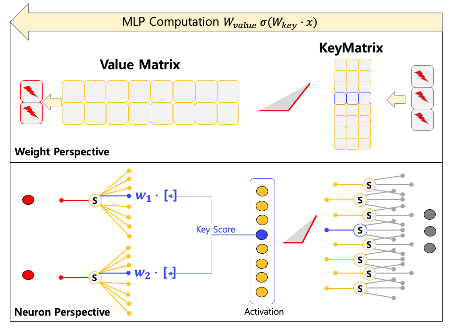
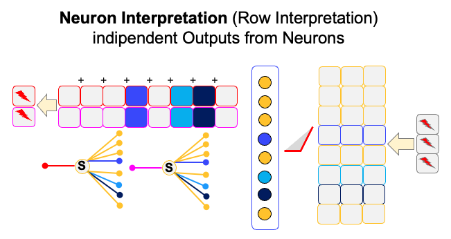
If we just assume that a neuron just provide a single output, we can interpret a neuron in a row-wise manner. That is, we don’t think about the meaning of weights and just consider the output value of each neuron. The Figure below shows the neuron-wise interpretation.
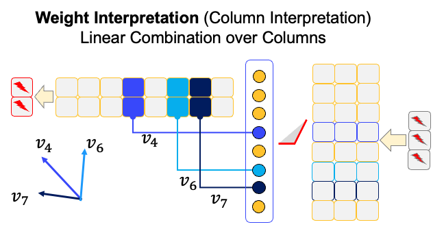
Unlike the neuron-wise interpretation where we interpret each neuron separately, we usually interpret multiple neurons together by considering the directional vector. In this case, the weights in value-neurons are not just used for aggregation of synapses, but could be interpreted by directionally meaningful information. The Figure below shows the example. In this case, the key is used to scale the vectors.