Deconvolution and Checkboard Artifacts
This is an informal review of a paper. We take computational analysis of convolution and deconvolution for artifact generation
Note: This post is a mathematical review of the paper “Deconvolution and Checkerboard Artifacts” [project link]
The motivation of this review is Circuits Thread
Introduction
The most widely used form of generative models is “Convolution - Deconvolution” structure. This structure has a bottleneck in the middle so that the compressed representation of an image can be encoded properly. At the stage of convolution layers, the information of an image is extracted. The stage of deconvolution layers recovers the image signals from the bottleneck representation by progressively widening the image sizes (normally double).
The impact of deconvolution has been studied by Odena et al. in the paper “Deconvolution and Checkerboard Artifacts” [project link]. The major problem is the overlapping signals from deconvolution operation. That is, deconvolution layers produce checkerboard artifacts in the output. Checkerboard artifacts are not representative features of an image because these are high frequency signals repeated locally which are unnatural representations. The interpretable reason of the checkerboard patterns is the deconvolution layer which spreads the input signals with convolutional filters. Note that deconvolution is a reverse operation of a convolutional layer which distributes the output signals to the input regions. In the process of distribution, the imbalance of signal distribution happens. To better understand the reasons of checkerboard artifacts, we analyze how convolutional and deconvolutional layers propagate the input signals. In addition, we review the “Resize-Convolution” which is an alternative operation for deconvolution.
Convolution and Deconvolution
We first analyze how convolution and deconvolution work
-
Convolution :
 Gathers the input signals : \((a,b,c) @ (x,y,z) \rightarrow (ax+by+cz)\)
 -
Deconvolution : Spreads the input signals : \((a) @ (x,y,z) \rightarrow (ax, ay, az)\)
See the Figures below for 1D examples.
🚀 Convolution and Deconvolution
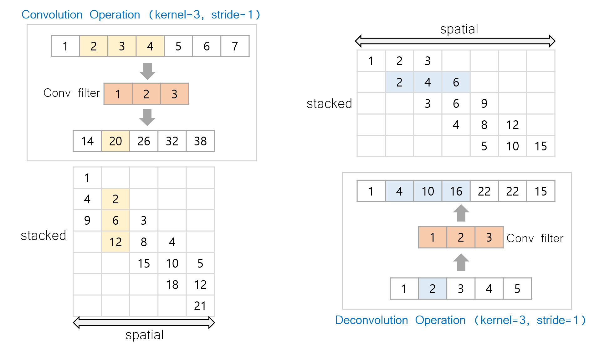
📌 Figure: (Left)
- Convolution Operation (
Kernel=3,Stride=1) - Pixels of
1~7are convolved with filter[1,2,3] - (Matrix) : For each pixel position, the accumulated signals are stacked.
📌 Figure: (Right)
- DeConvolution Operation (
Kernel=3,Stride=1) - Pixels of
1~5are deconvolved with filter[1,2,3] - (Matrix) : For each pixel position, the accumulated signals are stacked.
Convolution
Convolution gathers the local input signals and sums them up. Therefore, if there is a strong signal, it is propagated safely. On the other hand, the weak signals are not propagated. The convolution operation also smooths the local regions with proper strides.
\[\begin{aligned} \begin{bmatrix} a & b & c \end{bmatrix} * \begin{bmatrix} x_1 & x_2 & x_3 & x_4 & x_5 \end{bmatrix} &= \begin{bmatrix} a & b & c \\ & a & b & c \\ & & a & b & c \end{bmatrix} \cdot \begin{bmatrix} x_1 \\ x_2 \\ x_3 \\ x_4 \\ x_5 \end{bmatrix} \\ \\&= \begin{bmatrix} a x_1 + b x_2 + c x_3 \\ a x_2 + b x_3 + c x_4 \\ a x_3 + b x_4 + c x_5 \end{bmatrix} \end{aligned}\]Deconvolution
Decovolution spreads the input signal to neighbor regions. Unlike the convolution which has preserves the signal magnitude in monotonic manner, the deconvolution can
- 👾 Spike on a local region
- 👾 Make checkerboard patterns
When we analyze the operation of deconv, we can see that the middle part sums three components. This difference with conv
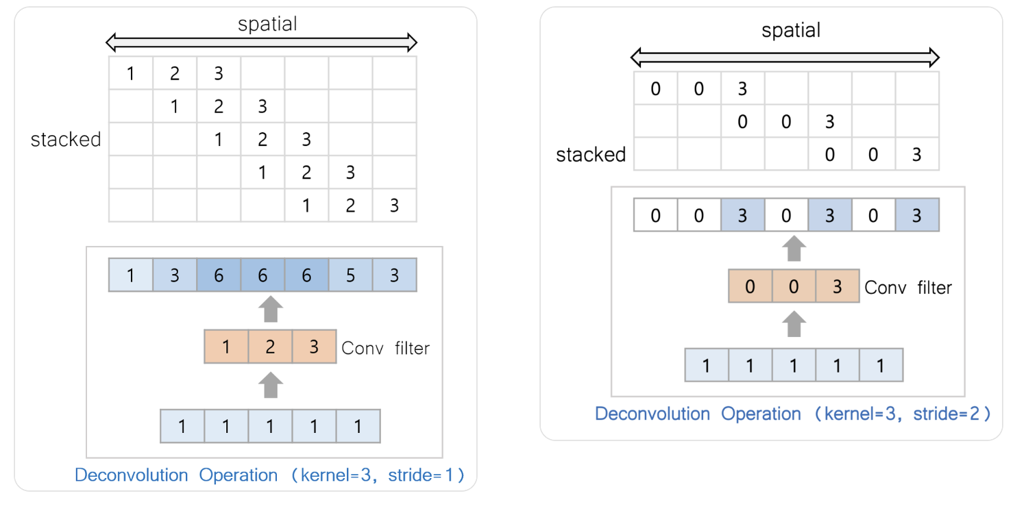
When we feed an uniform input signals $[1,1,1,1,1]$, we can observe how the signals are propagated through the deconvolutional layer.
🧙♂️ Problems of Deconvolution
Assume that we feed uniform signals $[1,1,\cdots]$
- Spike (left)
- Checkerboard (right)
Resize Convolution
The checkerboard artifacts suggest that we have to handle the proper stride and kernel size for better signal propagations. However, a more simple solution is avoiding deconvolution. Instead we can we just “Convolutional Layer” for the generation parts. The underlying assumption would be
It is easier to compress information, then spreading information
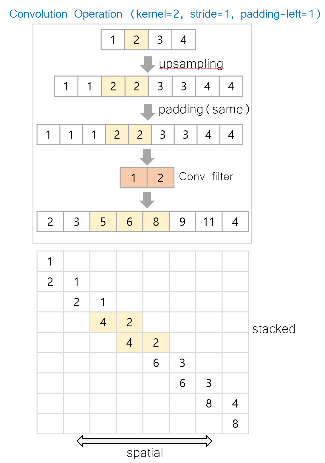
Therefore, the authors upsamples the original input and apply convolutional operation to decode the information in the easier way. If we follow the operation with a simple example (see the Figure below), we observe that the magnitude of an input signal is monotonically aligned with the output signal. With upscale (double) and padding for preserving the shape, we can ensure that the latent size progressively increases.
🚀 Resize Convolution
Resize-Convolution Parenthesis is image size (channel, width, height)
- → (C, H, W)
Image - → (C, 2xH, 2xW)
Upsampling - → (C, 2xH +a , 2xW + a)
Padding - → (C, 2xH, 2xW)
Convolution
Experimental Results
For experiments, the authors show that the inclusion and exclusion of deconvolutional layer is the main reason of the checkerboard artifacts and Resize-Convolution only shows no artifacts!

[Resize Convs ...] - [Deconv] - [Deconv]
When the last two layers are devons, the checkerboard patterns are visible

[Resize Convs ...] - [Deconv]
When the last layer is devon, the checkerboard patterns are visible. This case has higher frequency than the first one.

[Resize Convs ...]
When we don't use deconv and replace it with Resize-Convolution, no checkerboard patterns are visible.
Conclusion
In this post, we review the paper Deconvolution and Checkerboard Artifacts [Distill] which found the reasons of checkerboard artifacts and proposed solutions for it. By reviewing this paper, we found that understanding the computational meaning of a module is important and the inductive bias could be wrong
- Insufficient Training
- Insufficient Dataset
- Memorization and not generalization, including overfitting
- Wrong Inductive Bias (Deconvolutional Layer)
For me, a researcher in the field of interpretable AI, the most important approach is the last one. Most of tasks mostly care the training performances and do not deeply interpret the operational meaning of modules.
Acknowledgement
This article is a personal review of Deconvolution and Checkboard Artifacts [link]. There could be a wrong statement as this is an informal review of the paper.