Non-negative Matrix Factorization (NMF)

This is a gentle introduction of NMF.

Introduction

Non-Negative matrix Factorization (NMF) is a kind of MF whose matrix is non-negative entries. NMF has been widely used in the field of recommendation systems where users generate a massive number of information in the system and administrators want to find the important components. Consider the following example to understand the underlying assumptions of NMF.

There are two items whose representations are $[1,0,0]$ and $[1,1,0]$.
User 1 may select both items once, User 2 may select only the second item once, and User 3 may select the first item three times. As a result, we have the following representations for users.

User 1 Representation : $[2,1,0] = [1,0,0] + [1,1,0]$
User 2 Representation : $[1,1,0] = 0\cdot [1,0,0] + [1,1,0]$
User 3 Representation : $[3,0,0] = 3\cdot[1,0,0] + 0 \cdot [1,1,0]$

When we stack the representations in rows, we observe the following form of a matrix

Now, our problem is the reverse problem of finding items by decomposing the matrix. In detail, we find the underlying components (items) and weights which represent how the users select the components.

User 1 : $w_{11} * \mathbf{c}_1 + w_{12} * \mathbf{c}_2 + \cdots$
User 2 : $w_{21} * \mathbf{c}_1 + w_{22} * \mathbf{c}_2 + \cdots$
User 3 : $w_{31} * \mathbf{c}_1 + w_{32} * \mathbf{c}_2 + \cdots$

Mathematically, When we have a matrix of size n $\times$ d where d is the dimension of items and $n$ is the number of users, we may want to discover the underlying fixed number k of components.

We can also stack $w$ and $c$ to represent the overall factorization.

\[M = \begin{bmatrix} 2 & 1 & 0 \\ 1 & 1 & 0 \\ 3 & 0 & 0 \\ \vdots & \vdots & \vdots \end{bmatrix} = \begin{bmatrix} - \text{user } 1 - \\ - \text{user } 2 - \\ - \text{user } 3 - \\ \vdots \end{bmatrix}_{n\times d} = \begin{bmatrix} - \mathbf{w}_1 - \\ - \mathbf{w}_2 - \\ - \mathbf{w}_3 - \\ \vdots \end{bmatrix}_{n\times k} \cdot \begin{bmatrix} - \mathbf{c}_1 - \\ - \mathbf{c}_2 - \\ - \mathbf{c}_3 - \\ \vdots \end{bmatrix}_{k\times d} = W \cdot H\]

Note1

The User 1 representation is the linear combination of component representations with weights. The symbol $\textcolor{blue}{k}$ represents number of elements linear combined.

\[\begin{bmatrix} \textcolor{blue}{- \text{user } 1 -} \\ - \text{user } 2 - \\ - \text{user } 3 - \\ \vdots \end{bmatrix}_{n\times d} = \begin{bmatrix} \textcolor{blue}{- \mathbf{w}_1 -} \\ - \mathbf{w}_2 - \\ - \mathbf{w}_3 - \\ \vdots \end{bmatrix}_{n\times \textcolor{blue}{k}} \cdot \textcolor{blue}{\begin{bmatrix} - \mathbf{c}_1 - \\ - \mathbf{c}_2 - \\ - \mathbf{c}_3 - \\ \vdots \end{bmatrix}}_{\textcolor{blue}{k}\times d}\]

Note 2

There are many solutions to decompose the matrix into two factors $W$ and $H$. That is, the reverse problem does not guarantee the uniqueness of components and there are several ways we can decompose the matrix into weight matrix and component matrix. Even though we build the matrix from user selections of items, there is no relationship between the items and the found components from the matrix factorization

Non-Negative Matrix Factorization (NMF)

Let $M \in \mathbb{R}^{n\times d }$ be a non-negative matrix and $k$ is the number of components that we obtain by factorizing the matrix $M$. The factorization results in two matrices, weights $W \in \mathbb{R}^{n\times k }$ and components $H \in \mathbb{R}^{k\times d }$.

\[M = W \cdot H\]

According to Sklearn [link], the objective is not only recovering the matrix with $W$ and $H$, but also regularizing two matrices.

\[\begin{aligned} L(W,H) &= 0.5 \Vert X -HW \Vert_{loss}^{2} \\ &+ (L_1 \text{ regularization on vectors of } W) \\ &+ (L_1 \text{ regularization on vectors of } H) \\ &+ (\text{regularization on Frobenius norm of } W) \\ &+ (\text{regularization on Frobenius norm of } H) \end{aligned}\]

NMF Toy Example

Let’s consider a simple toy data for NMF. We have three four items: pizza, chicken, burger, and fries with the assumption that fries are always provided with a burger. Therefore, we have logically only three items even though the representation is four dimensional vector.

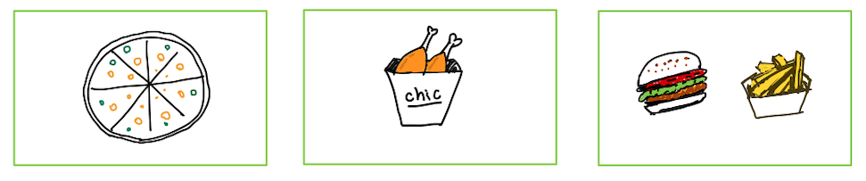
Note that it requires three items to represent the choice of a user, but four dimensions to represent physical items.

Pizza : $[1,0,0,0]$
Chicken : $[0,1,0,0]$
Burger+Fries : $[0,0,1,1]$

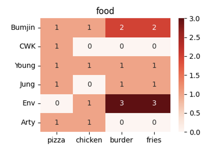
Now, there are multiple users who buy foods that they like.

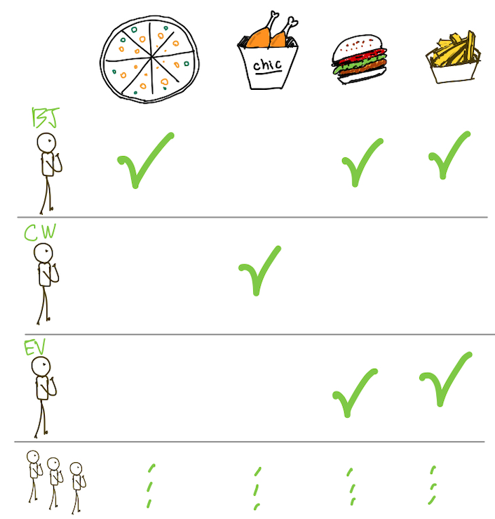
As the users can buy multiple foods, we can further make a toy matrix with weights.

blue color : a person bought two packs
red color : a person bought three packs

\[M = \begin{bmatrix} 1 & 1 & \textcolor{blue}{2} & \textcolor{blue}{2} \\ 1 & 0 & 0 & 0 \\ 1 & 1 & 1 & 1 \\ 1 & 0 & 1 & 1 \\ 0 & 1 & \textcolor{red}{3} & \textcolor{red}{3} \\ 1 & 1 & 0 & 0 \\ \end{bmatrix}\]

We can visualize the matrix with red colors.

NMF Result

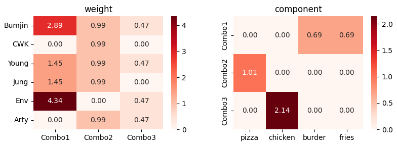
When we run the NMF with Sklearn, we have the following result.

\[M = W (\text{weight}) \cdot H (\text{components})\]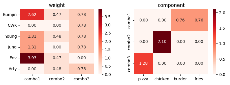

We can clearly see that components are one-hot vectors, but the magnitudes of components are not equal to 1. In addition, every component has different magnitude unlike the designed items of our toy food designs. In addition, when we run the algorithm with different seed we have different results.

Run Again…

It suggests that the iterative optimization in Sklearn does not provide a unique solution for NMF. However, we conjecture that correlated features are coupled when matrix is factorized (see burger and fries locations in columns 3 and 4 in component matrix). We can clearly see that two entries are in the same component.

Discussion

There are several questions when I learn NMF.

Are all elements of weights and components matrices zero? [ T / F ]
In which matrix should be encourage sparsity [ W / H / Both ]
Why should we decrease the Frobenius norm?
With permutation and scaling, all NMF results are similar? That is, how many distinct NMF results with permutation and scale invariance.