Understanding VQVAE

Description of VQVAE

1. Introduction

Auto-Encoders are recently developed by the progress of deep learning. Auto-Encoder learns the low-level representation of input data based on reconstruction objective. Auto-encoders are widely used to reduce embedding size or to get common vector size for the different types of input. One succesful advance is Vector-Quantized Variational Auto-Encdoer (VQ-VAE) which learns fixed length codes to represent input. VQ-VAE is used in D-ALLE, which is a text-guided image auto-regressive model, to represent an image as tokens. The procedure of VQ-VAE includes replacing an encoded latent vector with the clostest vector in the codebook. Even though the mechanism is simple, it is hard to implement it in differential manner and understanding the overall loss function. In this experiment, we discuss the forward and the backward flow of VQ-VAE and the effect of number of codes in the codebook.

2. Forward Pass of VQ-VAE

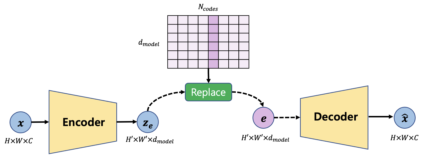
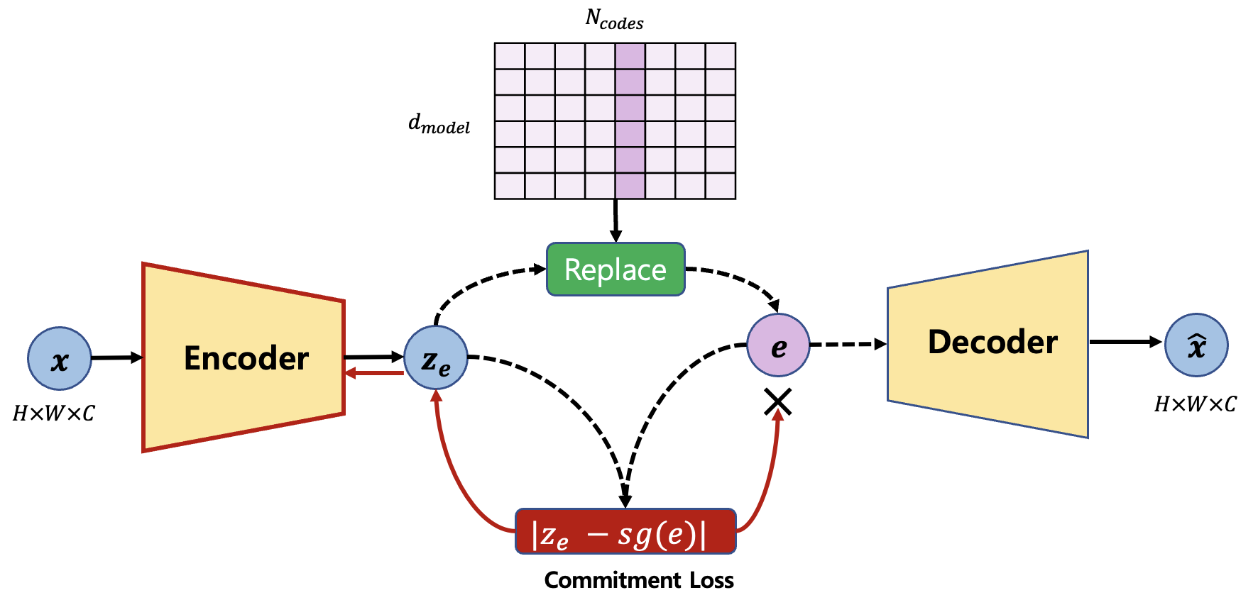
Figure 1 shows the forward pass of VQ-VAE. There are three modules: encoder, decoder, and quantizer. The encoder maps input $x$ to $z_e$ which is low-dimensional representation of $x$. Then the quantizer replaces $z_e$ with the closest vectors $e$ in the codebook. Finally, the decoder maps $e$ to $\hat{x}$ to reproduce the input. For example, $x$ of size 32x32x3 becomes 12x12x128 and each 12x12 vectors of size 128 is replaced with closest vector e of size 128 in the codebook. When there are K number of codes, the computation requires 12x12xK iteration to construct replaced codes.

Figure 1. The overall structure of VQ-VAE forward pass encodede latent $z_e$ is replaced by the closest latent $e$ in the codebook

3. Backward Pass of VQ-VAE

The objective is defined by

\[L = \log p(x|z_q(x)) + ||sg[z_e (x)] - e||_2^2 + \beta||z_e (x) - sg[e]||_2^2\]

The first is the reconstruction loss
The second term is for updating dictionary,
The third term is commitment loss to make sure the encoder commits to the output.

$sg$ represent stop gradient, that is, the value does not consist of computational graph. For example, $||y-\theta x+sg[\theta^2 x]||$ is just a linear function of $\theta$ because $sg[\theta^2 x]$ does not backpropagate.

in the original paper, they used $\beta=0.25$

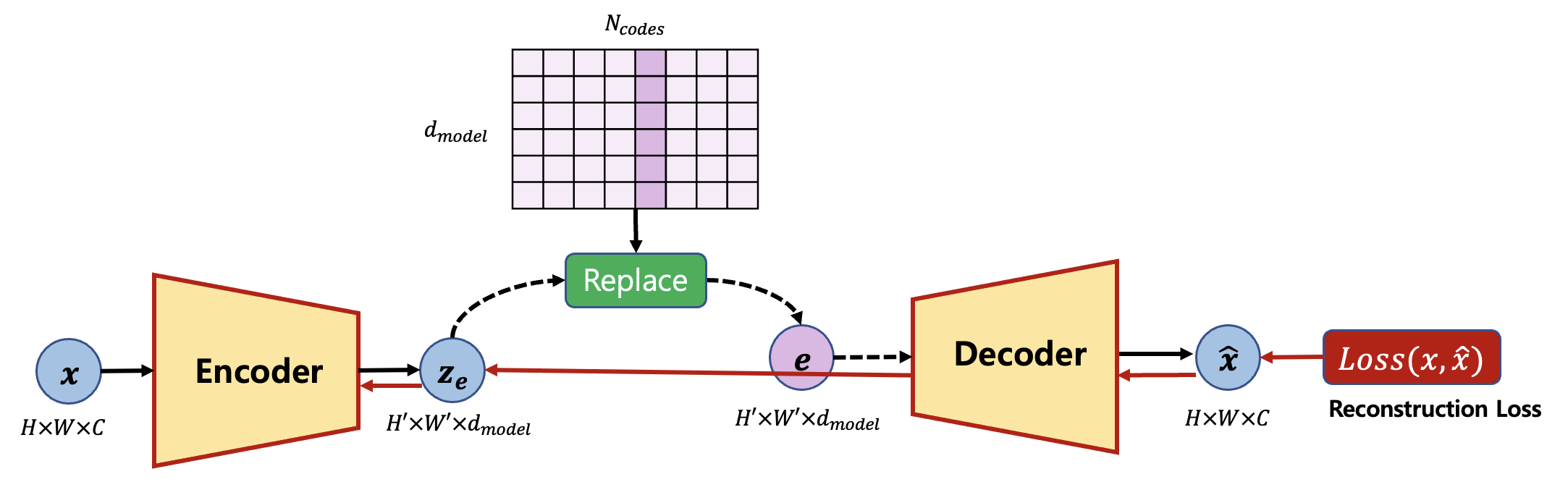
Loss 1 : Reconstruction

$L_{recon} = \log p(x|z_q(x))$

The reconstruction loss first flows to the decoder, and then encoder. In the implementation the replaced codes are not attached to the computational graph. Therefore, we have to replace $z_e$ vector with values of $e$ by the code below.

quantized = quantize(input) input = input - (input.detach() - quantized) # detach means, stop gradient # input.item() = quanized.item()

Figure 2. The backward pass of the reconstruction loss. The red lines represent the computational paths and the edges of red lines are updated modules

Loss 2 : Dictionary

$L_{dict} =||sg[z_e (x)] - e||_2^2$

The dictionary loss is defined to match the dictionary representation with the encoder representation. As can be seen in Figure 3, the gradient does not flow to the encoder and flow only to the decoder. In the paper, this loss is higher ($\beta=0.25$) to make the encoder representation follows the dictionary representation, that is, the dictionary update is faster.

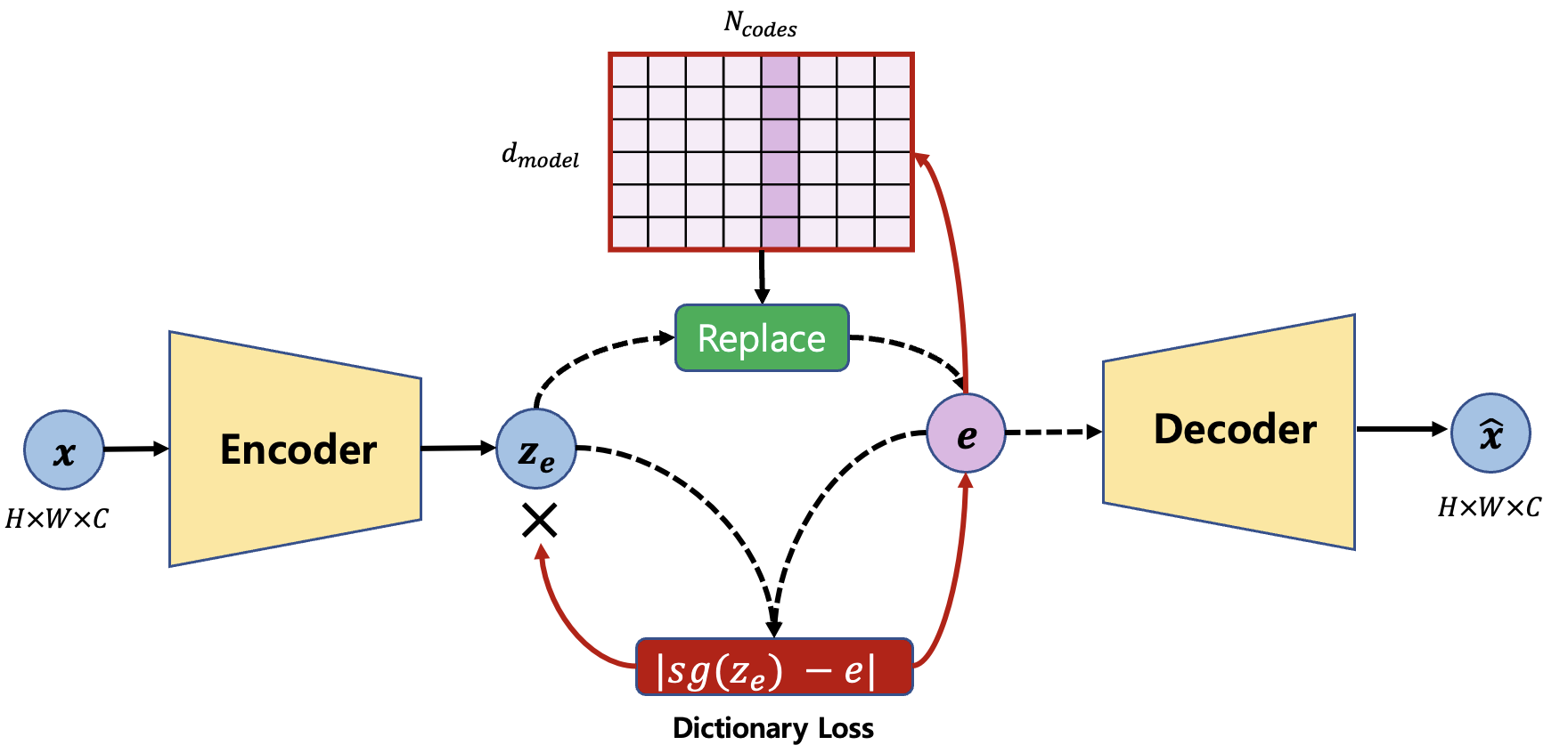
Figure 3. The backward pass of the dictionary loss. The red lines represent the computational paths and the edges of red lines are updated modules

Loss 3 : Commitment

$L_{commit} = \beta||z_e (x) - sg[e]||_2^2$

The commitment loss is defined to match the encoder representation with the dictionary representation. As can be seen in Figure 4, the gradient does not flow to the dictionary and flow only to the encoder.

Figure 4. The backward pass of the commitment loss. The red lines represent the computational paths and the edges of red lines are updated modules

4. Experiment

Model Structure

VQVAE( (encoder): Encoder( (net): Sequential( (0): Conv2d(3, 32, kernel_size=(4, 4), stride=(2, 2), padding=(1, 1)) (1): ReLU() (2): Conv2d(32, 64, kernel_size=(4, 4), stride=(2, 2), padding=(1, 1)) (3): ReLU() (4): Conv2d(64, 128, kernel_size=(4, 4), stride=(2, 2), padding=(1, 1)) (5): ReLU() ) ) (decoder): Decoder( (net): Sequential( (0): ConvTranspose2d(128, 64, kernel_size=(4, 4), stride=(2, 2), padding=(1, 1)) (1): Tanh() (2): ConvTranspose2d(64, 32, kernel_size=(4, 4), stride=(2, 2), padding=(1, 1)) (3): Tanh() (4): ConvTranspose2d(32, 3, kernel_size=(4, 4), stride=(2, 2), padding=(1, 1)) ) ) (before_quantize): Conv2d(128, 256, kernel_size=(4, 4), stride=(2, 2), padding=(1, 1)) (quantizer): Quantizer( (codebook): Embedding(256, 256) ) (after_quantize): ConvTranspose2d(256, 128, kernel_size=(4, 4), stride=(2, 2), padding=(1, 1)) )

Hyperparameter Tuning

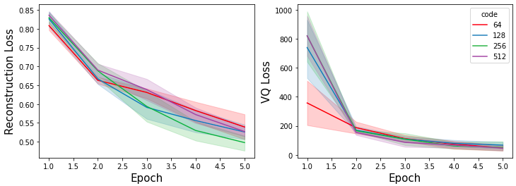
The performance of VQ-VAE depends highly on the number of codes in the codebook and the size of latent vectors. If ther are two many codes, the shared latents are sparse. Therefore, we train VQ-VAE with differnt hyperparameters [64, 128, 256, 512] for both the number of codes and the size of latent vectors. The Figure 5 shows the trend of reconstruction loss and VQ loss. The reconstruction loss of 256 codes showed the fastest decrease.

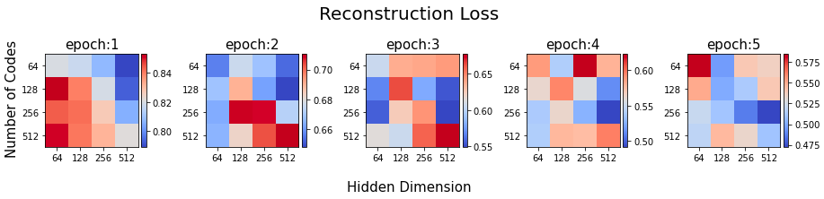
Figure 5. Reconstruction loss while training for 64,128,256,512 codebook sizes and hidden dimension

The Figure 6 shows all pairs of reconstruction loss. 256-256 was the best.

Figure 6. Training loss for codebook sizes. The 95R% confidence regions are colored.

Full Training with (256, 256)

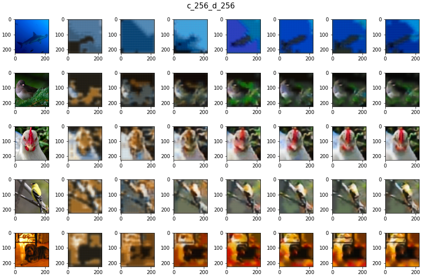
The Figure 7 shows reconstructed images with 256-256 pair in the early stage. The images are trained to match overall structure but fail to reconstruct details.

Figure 7. VQ-VAE reconstruction in the early stage. The training captures the overall structure first. Details and color of the image are captured later.

With the result of hyperparameter test, we train the model further. As shown in the Figure 8, VQ-VAE now reconstruct colors and details of the images.

Figure 8.VQ-VAE reconstruction for all training iteration.

5. Conclusion

The performance of VQ-VAE depends on the codebooks. It is better to tune the number of codes for abstraction and divergence of representation. Single forward uses $\mathcal{O}(HWK)$ computation time for selecting the clostest code where $H,W$ are width and height of the latent representation, and $K$ is the number of codes. Therefore, the three sizes must be properly reduced. Two aspects are not considered in this experiment.

1) How the encoder and the decoder affect performance?

2) What happens if training is done further with small nubmer of latent codes?

Even though the reconstruction error is higher, may be it is better to have shared latent codes for all images.